Most common PC image files that we are likely to encounter (JPG, GIF, TIFF etc...) support only 8-bit grayscale. They may encode millions of colors, but only support 256 shades of gray. Also, current "24 bit" PC video card technology is incapable of displaying more than 256 shades of grays on the monitor. There is no great incentive to display more than 256 shades of gray since human vision can only resolve about 32 to 64 shades of gray.

For Medical Imaging purposes this display range is not sufficient to differentiate the subtle differences between some tissues. CT and MR imaging, for instance, can resolve differences in tissue properties of one part in several thousand. The pixels of a CT image, for example, are proportional to tissue electron density and are usually expressed in Hounsfield Units, which roughly cover the numerical range -1000 to +1000. A medical image pixel is usually stored as a 16-bit integer. Two industry standard file formats that support 16-bit data are DICOM and TIFF. Madena has the capabilty to import both these image formats.

The 16-bit medical image is capable of storing a much wider dynamic range of information than can be displayed on a PC video monitor. This is usually resolved by compressing the 16 bit data from a user defined display range (the "window") to 8 bit (256 shades of gray.) Madena provides Window & Level functionality in three ways:

1. A dialog which displays a histogram of the image density distribution. In this dialog you can select the range of 16 bit data to compress and a compression function. The function which is commonly associated with "window & level" in medical imaging systems is a linear gradient between "black" and "white". In Madena, the compression function can be either linear (modified by brightness & contrast controls) or non-linear (modified by bias and gain controls). The dialog is accessed from the WIN+LEV button. This button becomes active if the program detects that the displayed image has 16-bit grayscale data.



2. Window & level settings can be selected from a contextual menu of up to 16 user defined presets by control-clicking (or click and hold for 2 seconds) on the button. The presets are defined in the preferences dialog.



3. "Window & level" can be adjusted interactively in an image window using the cursor (eg. mouse). Click the small "window & level" icon button at the bottom of the image window (next to the magnification buttons). The cursor will change to a window & level symbol when it is over the image. Click & drag the cursor on the image. Dragging the cursor (ie mouse) left & right on the screen adjusts the midpoint of the displayed range (the "level"). Dragging up & down on the screen adjusts the width of the displayed range (the "window"). When you are satisfied with the image appearance, click the icon button at the bottom of the image window again to exit "window & level" mode.

Window & Level Dialog



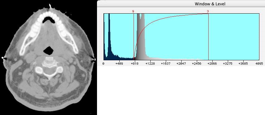
When you click on the Window & level button, an Interactive dialog is displayed which consists of the following:

1. Histogram. The histogram displays the image data as a function of numerical pixel value. Peaks represent values with large pixel counts (eg. large areas of uniform density, such as air or soft tissue).


2. Raw data range section This is the subrange of data found in the image file. A CT image might be stored as signed 16-bit integers (-32767..+32767) but the useful data may only occupy a subrange (0..2000). There is usually no reason to change these values. Any pixels outside the raw data range are ignored.


3. Display range section

   The original concept of window & level evolved from CT imaging and has historically expressed the range of displayed data as the absolute value of the difference between the highest and lowest numerical pixel values (eg. Hounsfield Units) to be displayed (ie the "window" width) and the numerical midpoint of that range (the "level"). The upper and lower display range bounds are therefore the level plus or minus half the window width. This method of expressing the display range is intuitive only if the compression fuction which converts the window to shades of gray is symmetrical around the "level". It also runs into symmetry problems at the extreme limits of the raw data range.

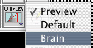
   In Madena, the window & level compression function can be nonlinear and asymmetric around the "level". Image data can have a wide variety of physcial interpretations. To keep the concepts as generic as possible, Madena's display range boundries are expressed as a fraction of the raw data range (absolute pixel values are also included for convenience above the editable text fields). The upper and lower boundries of the display range are marked by two vertical red lines on the histogram, joined by a graph of the compression function. You can adjust the display boundries by typing numbers, clicking on the "little arrow" bumpers, or dragging the red lines on the histogram. The Preset menu allows you to quickly choose between 16 user defined window & level settings. Each preset includes the display range bounds, brightness, contrast, bias, gain, gain midpoint (M) and a few other parameters (see preferences dialog). The presets (except for the 1st preset which is reserved for file preview use) can be assigned menu names via the preferences dialog.



4. Profiling range section

   Measured pixel profiles are plotted as pixel density on the Y axis versus pixel location on the X axis of the graph. The Y axis plot range defaults to the raw 16-bit data range of the image but can be changed here to cover the display range or an arbitrary (custom) range of densities.



5. Zoom Control The zoom control affects only the vertical scaling of the histogram. Use this control to see detail that would otherwise be obscured by the peaks.



6. Brightness, Contrast (Bias, Gain) Controls These controls affect the compression function that maps raw 16-bit data into the 8-bit display range. The Gamma button switches between the linear bright/contrast and nonlinear bias/gain compression functions. The "M" slider shifts the gain point. All of these functions default to the midpoint (0.5) of the sliders. The "Reset" button returns all sliders to their defaults. The "Reverse" button switches the mapping of density to grays. Usually, the lowest density value in an image is displayed as "black" and the highest as white (this corresponds to the DICOM MONOCHROME2 file type). You can reverse this if you wish so that low densities appear as "white" and high density values display as "black" (eg. the DICOM MONOCHROME1 file type). Note: the compression contrast should always be set to 0.5. In general, it's better to use the image window controls to change brightness and contrast rather than the compression controls. The bias and gain functions are more useful as compression modifiers.

   Below is an example of nonlinear compression using bias and gain.

   
   

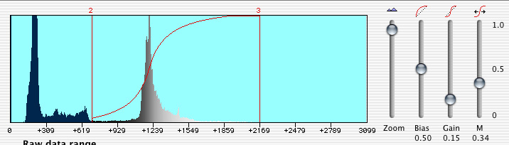
   The CT image of a shark head (from the recent SciFi movie "Deep Blue Sea") on the left was created using linear compression, the image on the right using the nonlinear bias and gain settings illustrated above.

   
   

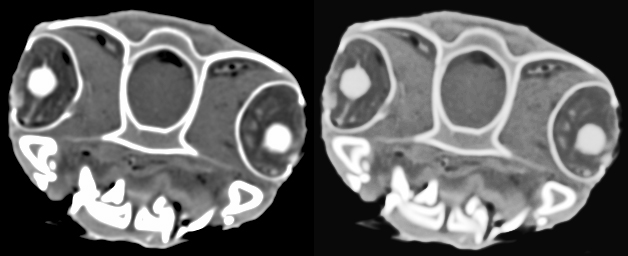
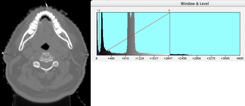
   In this next example, a CT slice through the jaw requires a wide "window" centered (level) on the soft tissue peak to see both soft tissue, jaw and teeth. In order to cover such a wide range of CT densities, there are few shades of gray available for the peak and thus little soft tissue contrast.

   
   

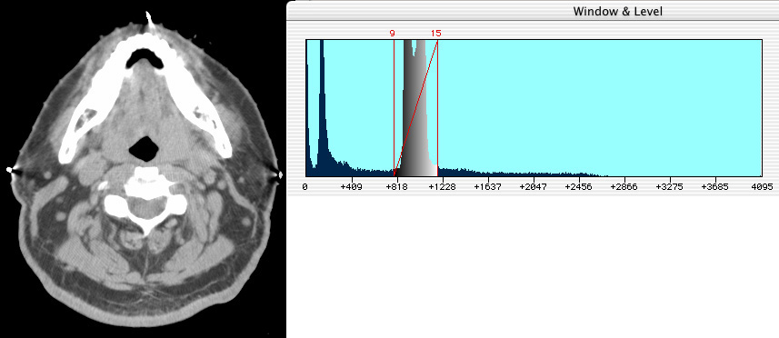
   This is an example of using a narrow window to get better soft tissue contrast on the peak, but the jaw and teeth are all mapped to "white" and have lost detail. As an analogy, if this were a photograhic film, you might say the jaw and teeth were "overexposed".

   
   

   This is an example of using bias & gain to maintain both some soft tissue contrast and some detail in the jaw and teeth.

   
   


7. Copy to Preset Prefs. This button copies the current settings (in normalized mode) to the preferences for the currently selected preset. You will need to save preferences to make the changes permanent. To create preset preferences in absolute (eg. Hounsfield Units) mode you must manually enter the display range bounds and set the mode to "Hounsfield Units" in the preferences dialog.